Statistical Graphics vs. InfoVis

The current issue of the Statistical Computing and Graphics Newsletter features two invited articles, which both look at the “graphical display of quantitative data” – one from the perspective of statistical graphics, and one from the perspective of information visualization.

Robert Kosara writes from an InfoVis view: 

Visualization: It’s More than Pictures!

Information visualization is a field that has had trouble defining its boundaries, and that consequently is often misunderstood. It doesn’t help that InfoVis, as it is also known, produces pretty pictures that people like to look at and link to or send around. But InfoVis is more than pretty pictures, and it is more than statistical graphics.

The key to understanding InfoVis is to ignore the images for a moment and focus on the part that is often lost: interaction. When we use visualiza- tion tools, we don’t just create one image or one kind of visualization. In fact, most people would argue that there is not just one perfect visualization configuration that will answer a question [4]. The process of examining data requires trying out different visualization techniques, …

read on in the Newsletter.

Andrew Gelman and Antony Unwin write from an statistical graphics view:

Visualization, Graphics, and Statistics

Quantitative graphics, like statistics itself, is a young and immature field. Methods as fundamental as histograms and scatterplots are common now, but that was not always the case. More recent developments like parallel coordinate plots are still establishing themselves. Within academic statistics (and statistically-inclined applied fields such as economics, sociology, and epidemiology), graphical methods tend to be seen as diversions from more “serious” analytical techniques. Statistics journals rarely cover graphical methods, and Howard Wainer has reported that, even in the Journal of Computational and Graphical Statistics, 80% of the articles are about computation, only 20% about graphics.

Outside of statistics, though, infographics and data visualization are more important. Graphics give a sense of the size of big numbers,  …

… read on in the Newsletter.

You will be surprised about the amount of consensus, as well as the topics of dispute – both might probably not match your expectation, but can be a start of an open discussion.

This blog post shall be the platform for this discussion and we are looking forward to reading your comments …
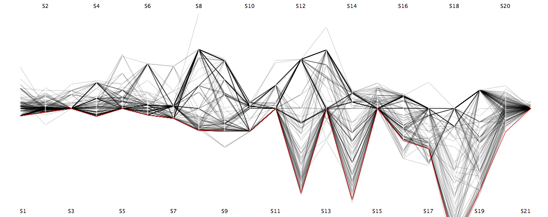
Tour de France 2011

— that’s it for this year, see you in 2012 (the latest) – au revoir! —
(With now 7 years of full Tour de France data, I might start to compare the different tours on a more “global” level.)

Again, the Tour de France has to compete with the soccer world championship – ok, this time it’s the girl’s turn and the attention is somewhat smaller …

Although I “missed” the first 5 stages, I will start to log the results in the usual ways as in 2005, 2006, 2007, 20082009 and 2010.

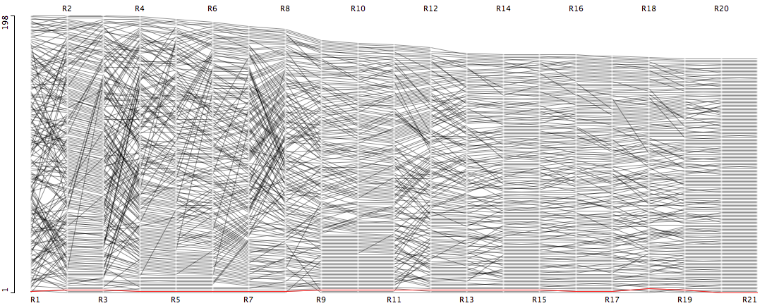
Stage Results cumulative Time Ranks
Stage Total Rank
(click on the images to enlarge)

– each line corresponds to a rider
– smaller numbers are shorter times, i.e. better ranks
– all stages are on a common scale,
– stage-results and cum-times are aligned at the median, which corresponds to the peloton

STAGE 6: Still a very compact group of 18 riders at the top of the field
STAGE 7: Easy riding
STAGE 8: The first mountains shrink the top group to 11
STAGE 9: Thomas VÖKLER now almost 2′ ahead
STAGE 10: No changes in the Top 42
STAGE 11: Still waiting for the Pyrenees
STAGE 12: Team Leopard-Trek lead by the SCHLECK brothers with 5 in the top 44
STAGE 13: Vincent JEROME lost hist last place for the first time
STAGE 14: Thomas VÖCKLER still almost 2” in front
STATE 15: Here are the 28 drop-outs so far, as the ranks almost stay unchanged
STAGE 16: HUSHOVD wins and TEAM GARMIN takes the lead
STAGE 17: The worse riders are all collected into the peloton
STAGE 18: Andy SCHLECK rushes (almost) to the top! Still 4 within 1′ reach!
STAGE 19: VOECKLER can’t defeat the SCHLECK brothers but still in reach
STAGE 20: EVANS too fast for Andy Schleck but not for MARTIN
STAGE 21: Congratulations to Cadel EVANS

(Note: The official results for stage 2 are missing, and thus are calculated from the differences of the total times)

For those who want to play with the data. The graphs are created with Mondrian.

There is a more elaborate analysis of Tour de France (2005) data in the book.

Of course – as every year – a big thanks to Sergej for updating the script!

A Design Classic demystified?

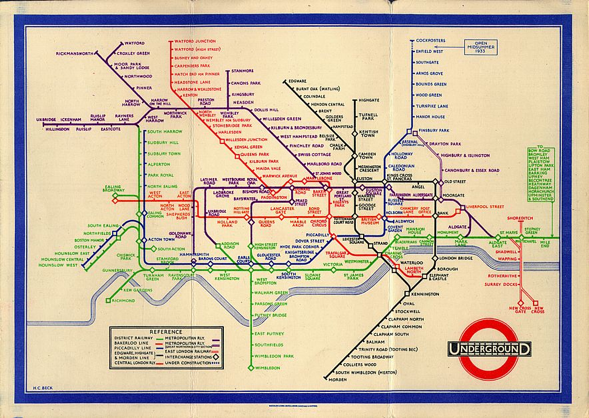
Mr. Beck’s London Tube map is a real design classic. Besides the timeless and universal design, the chosen geographical distortion has always been a point of discussion.

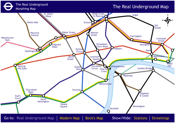
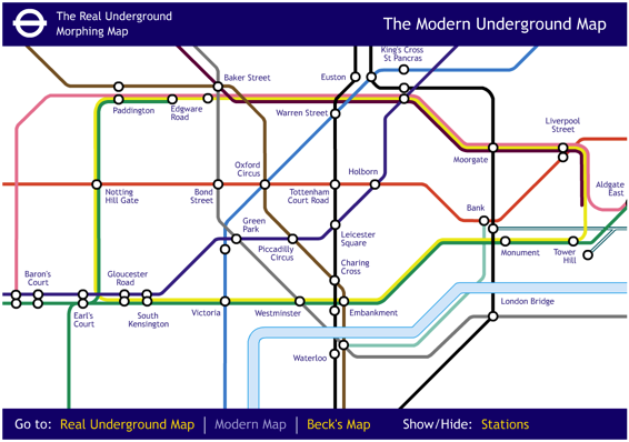
At fourthway [via infosthetics] we find a nice animation between the “real map”, which is geographically correct and the stylized map, which is optimized for reading and aesthetics.

Here are the two versions:

At first glance, the very nice animation might give us the impression that Beck’s creation is really of no help as the geographically correct map is still nicely readable and gives us so much more insight of where we actually are or go.

So did Beck err, and we are being fooled by strange subway maps around the world for no reason? Certainly not!

The answer is quite simple. The clip the guys at fourthway use is a quite small part of London’s inner city. Thus the average distance between stations has a relatively small variance (and is small itself), and – as we see – it does not make much of a difference which version of the map we look at.

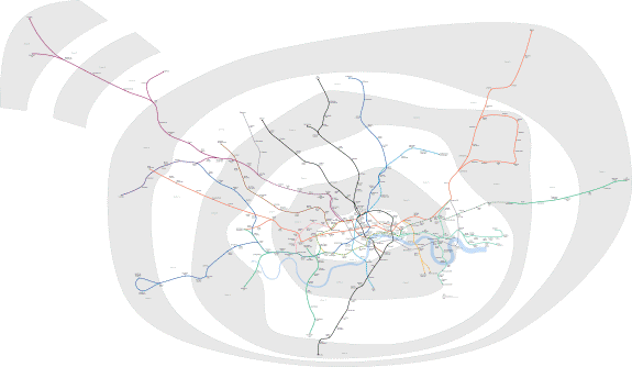
Taking the current complete map and shading the chosen clip in it, shows how much of the subway network is not covered:

I am too lazy now to get the real distances fixed, but only looking at the fare zones (as a proxy for distance) shows us that the clip covers mainly only fare zone one, and almost any line extends to at least zone 4, some even as far as 9.

The full story of a geographically correct London Tube map looks like this

and can be found at Wikimedia along with some more detailed maps.

Now it is very easy to understand why Mr. Beck really had a brilliant idea in choosing this particular design which was consequently adopted in subways around the world.

R GUIs: Which one fits you?

The gap of the new “digital divide” between those who only use computers when they are as easy to use as iPads and smartphones and those who like (or at least accept) to type commands to perform jobs, seems to get bigger and bigger.

R – the lingua franca of statistical computing – is exactly such a command-line based language, reasonably well designed but still not GUI based at all. At this point GUIs are the only solution to make R accessible for “generation point-and-click” and bridge the divide.

Personally, I am happy to use all well designed GUIs but as well see the power of language based command line interfaces – you need to work with both to be most effective.
But let’s come to the comparison of the four different frontends for R (in lexicographic order) which try to do more than the built-in standard GUIs for the supported platforms:

(mouse-over the entries in the table to get more details)

JGR

RCommander

RKWard

R Studio

Technology JAVA tcl/tk KDE Qt
Platform
Installation simple simple painful easy
Approach IDE comprehensive comprehensive IDE
Interface SDI MDI (plus R) TDI MDI
Maturity 1.7-5 1.6-3 0.5.5 0.92.44
Console yes yes yes yes
CodeEditor yes no yes yes
Objbrowser yes no yes yes
DataEditor yes via fix() yes no
ModelBrws yes no no no
Logging console console extended console
Plugins via iWidgets yes yes no
Web-Client no no no yes

There are certainly more frontends and features (especially on the technical side) to consider, and not everybody will share my verdict on every point (which I even probably didn’t get completely right), but that’s what comments are for  …

My summary recommendations (regarding the four candidates) are:

  • working styles are very different such that many of the above mentioned issues may be pointless
  • for many of us the built-in GUIs are pretty good already, but differ from platform to platform (so you maybe want to avoid any further hassle)
  • if you are on a Mac, half of the choices are gone already …
  • those who really don’t like to “being helped” by your software, opt for the IDE approaches!
  • those who really don’t want to learn any of the R-syntax and are purely on a user level, use one of the comprehensive approaches – you still might not be too happy though
  • if you hate installation procedures, make sure to avoid RKWard (under Windows)
  • the sleekest GUI is definitely R Studio
  • if the webpage would be wider, I should have certainly mentioned Deducer, which is a comprehensive offspring of JGR.

Japan Earthquake: An Exploratory View

Thanks to the data provided by the USGS, we can take a look at all earthquakes since 1973, which cover almost the last 40 years of earthquake activity worldwide.

Let’s first take a look at the yearly development of the earthquake activity overall:

The apparent increase in the last 10 years is striking – though I don’t have any explanation for this change, which is most probably not even man-made. Interestingly the magnitude (see next figure) does not increase, though the chance of stronger earthquakes will grow with the overall number.

The distribution of magnitudes (which is used for the coloring) is even more striking, looking at the earthquake in Japan, March 11th which is now rated as a 9.0.

The whole dataset contains only one earthquake at a higher magnitude, i.e., the earthquake originating the terrible tsunami on the 2nd Christmas day in 2004 at a magnitude of 9.1.

Keep in mind that the Richter scale is logarithmic, i.e., stepping up one unit means a 10 times stronger earthquake. The strongest ever measured earthquake was in Chile in 1960 at 9.5.

If we look at the coordinates of the measurements in longitudes and latitudes, we see how much the activity is concentrated on the tectonic hotspots.

We roughly see the shapes of some continents, with one exception. Africa seems to be free of any activity; probably due to the fact that it sits happily on its own tectonic plate.

Looking at this data, we can only start to understand the devastation Japan is facing.

(The data can be loaded directly into Mondrian, which was used to create the graphs above.)

The Good & the Bad [3/2011]

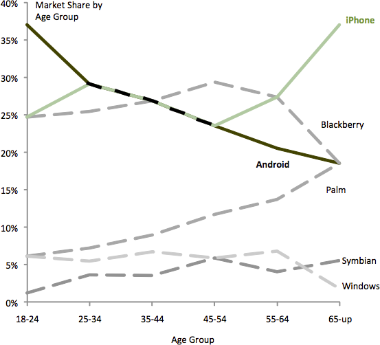
This post could as well be called “Which Smartphone is right for you?”, or “Plotting conditional distribution – but the right way!”. Here is the original visualization from Nielsen, which is not really bad, but still hides the important message to some extent.

Kaiser adequately pointed out that some features – important features – of the data are hard to spot in the Nielsen graphic. His improved version does not use areas any more, but shows the shares of the different OSs as lines over the age axis.

From this display we may conclude two things:

  1. Areas are unsuitable to display this kind of data
  2. We understand the data better when we condition on age instead of OS
    (it somehow seems more natural that given a particular age, we might choose a certain phone and not vice versa)

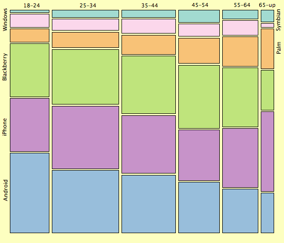
Thanks to Kaiser who shares the data on his blog, I was able to create the “rotated” mosaic plot, which also conditions on age but still uses the proportional areas.

We clearly see that not the areal 2-dimensional representation is the problem, but the conditioning was just chosen the wrong way. In this representation we also can retain the overall sizes of the groups, which is an advantage over the line plot.

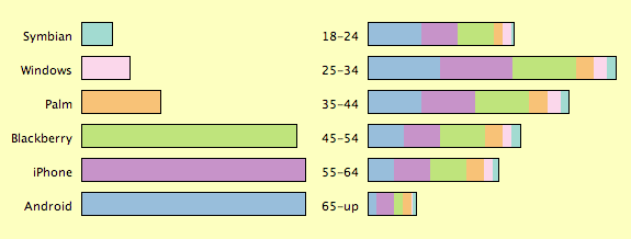
Things are even easier to interpret to with the marginals as legends:

From this mosaic plot we can perfectly read some of the features of the data:

  • the popularity of Android phones decreases with age
    (maybe because they are cheap and tailored towards tech-oriented people)
  • iPhones and Palms show an increasing popularity for ages above 55, and
    (probably due to an interface more suited for “ordinary” people)
  • vice versa Windows and Blackberry are underrepresented for 55+
    (maybe they are no longer being forced by their employers to use these phones)

(Graphs were made with Mondrian)

Too Hot to handle?

This is the ideal post to combine Infographics/Visualizations with the user interface aspect. I found it on Kaiser’s Junk Charts.

Having spent only a few years of my life in the US and being inculturated in orderly and standardized Germany, I can tell that most faucets here come pretty close to the “should be” situation. This is mainly due to the fact that we handle temperature and water flow in two or more, but separate dimensions. The combined interface is as wired as hard to handle. My impression though is that the “magma” range is as wide as the “ice cold”, what does not change the problem at all.

Nonetheless, once you took a shower in the US, you know what it means to find this tiny slot between “ice cold” and “magma” – and for the non-US readers, I really mean “magma” not just “hot water” ;-). Thanks to the creator of this fun graphics!

Visualizing Soccer League Standings

I feel ashamed for this boring title, but hope that the entry can make up for it. This visualization did inspire me, as a comment did point to my Tour de France visualizations.

As with all visualizations, we need data first – this sounds trivial, but is sometimes a frustrating show-stopper. After I found the Bundesliga data for each round, the only thing missing was the script to pull the data off the website. R‘s xml-package was the choice:

library(XML)
games = 23
for (i in 1:games) {
   url = paste("http://www.sport1.de/dynamic/datencenter/sport/ergebnisse/
                fussball/bundesliga-2010-2011/_r10353_/_m",i,"_/", sep="")
   rawtab = readHTMLTable(url)
   tab = rawtab[[6]][3:20,c(2,9)]
   ids = order(tab[,1])
   if( i == 1 )
     result = tab[ids,]
   else
     result[,i+1] <- tab[ids,2]
}
resdf <- as.data.frame(result)
names(resdf)[1] = "Team"
names(resdf)[2:(games+1)] = 1:games
write.table(resdf, "Bundesliga.txt", quote=F, row.names=F, sep="\t")

Although I didn’t use readHTMLTable before, it was a 15 min. job to get the script fixed – a definite recommendation for jobs like this!

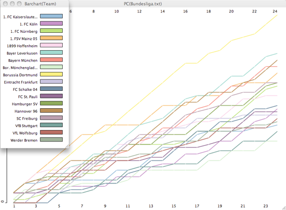
But now to the visualizations: Let’s start with the simple trajectories of the points of each team.

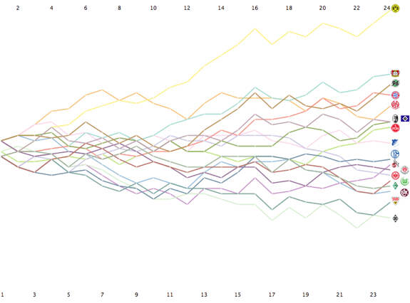
As one of the comments on reddit already suggested, we might want to align the developing scores along the median:

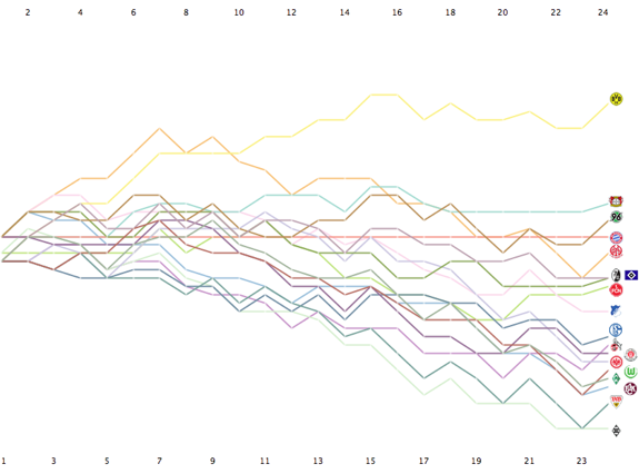
Now, as this weekend the “Rekordmeister” – as the FC Bayern names itself full pride – lost at home against BVB 1:3, it might be worthwhile to look at the scores from a FC Bayern perspective, i.e., we align the scores at the result from the FCB:


Easy to see that the gap to BVB remains at the same level for more than 10 games now, and for roughly five games, the direct opponents are somehow not to get rid off.

Here is the text file, you might use to play around yourself using Mondrian – which was used to create the visualizations.

Advertising and Statistics

There is certainly a prerequisite for statistics we can’t get around: data. Online advertising services generate tons of it; most not accessible for the public and many probably not very interesting at all.

Chitika has made one statistics public for us: the penetration of iPhones on the AT&T and Verizon network

We don’t get any info on how the data is measured (iPhone versions, representative placement of ads, …) and (unfortunately) there is no historic data, i.e., a time series.

Nonetheless, verizon is catching up quite fast, and I bet the CEOs of competitor networks in other countries Apple finally opened up, would die to get these figures for their networks …

Statistical Computing and Graphics Newsletter

The new issue (Vol. 21, No. 2) is out now. Featured articles are:

barNest: Illustrating nested summary measures
by Jim Lemon and Ofir Levy

You say “graph invariant,” I say “test statistic”
by Carey E. Priebe, Glen A. Coppersmith and Andrey Rukhin

Computation in Large-Scale Scientific and Internet Data Applications is a Focus of MMDS 2010
by Michael W. Mahoney

and of course, announcements and the news from the section chairs.

Andreas Krause passed the graphics editorship over to me last fall, and I am looking forward to a lot of interesting submissions in the coming years.

Please feel free to contact us (Nicholas, computing co-editor, or me, graphics co-editor) no matter whether you are a student or professor, a statistician or a practitioner, … whatever is interesting to the community and has its quality has a pretty good chance to be published.

Data Analysis of Yesteryear

It is not too often that a book is published that integrates data analytical methodology and the illustration of the appropriate use of specific tools. When Henk pointed me to the just released “Data Analysis with Open Source Tools” by Philipp Janert, the excitement was big, but it evaporated as soon as I read through the book.

I did start to flip through the pages with Amazon Preview, and was positively surprised that Part I of the book was on “Graphics: Looking at Data” and the following sections were actually progressing in the dimensionality of the data looked at – nice concept, and well copied. The first figure though, is a jittered dotplot – something we were doing in the 70s when we were still sending our plot commands to a pen plotter, and were trying to avoid ink soaked holes in the paper – we should know better more than a quarter of a century later.

It takes quite some pages until the book hits the widely used boxplots in the section “Only when Appropriate: Summary Statistics and Box Plots“, and we read “These summary statistics (mean and median, standard deviation, and percentiles) apply only under certain assumptions and are misleading, if not downright wrong, is those assumptions are not fulfilled.” Well, how can a median be wrong?

A surprising highlight can be found on page 68, where Janert absolutely hits the point in the distinction between “Graphical Analysis and Presentation Graphics” – something he seems to have forgotten just 50 pages later.

In the section on multivariate data analysis Janert talks about “Interactive Exploration” and writes “Now I could imagine a tool that allows us to select a bin in one of the histograms and then highlights the contribution from the points in that bin in all the other histograms“. His imagination could come true with a few clicks when he would use the appropriate tools. On page 124, he throws ggobi and Mondrian in the subtly named group of “Experimental Tools“. He claims “I don’t think any of these novel plot types have been refined to a point where they are clearly useful.” Certainly, if you do not use these (novel?) plots – btw. PCPs had their 25th anniversary last year and mosaic plots will celebrate their 30th anniversary this year – you wont see their usefulness. That Janert most likely did not use Mondrian is somehow apparent, otherwise he would not need to imagine a tool that links histograms.
The last lowlight to present here  is the “histogram” in Figure 9.4 on page 202, which is – hey – just a scatterplot; they are not that hard to tell apart.
I hate being so critical, but we should not let someone get away with a book on data analysis published in 2010 bashing what is standard in modern, interactive, graphical data analysis for more than a decade now. Who would consider using Gnuplot for graphical data analysis in 2011?

If you answer above question with “yes”, go buy the book – if not, save the money for a more up-to-date book.

Mondrian Version 1.2 released

The new version (1.2) of Mondrian adds the following (significant) features:

  • Scatterplotsmoother now includes “principle curves“, which are one of the nonlinear generalizations of principal components.
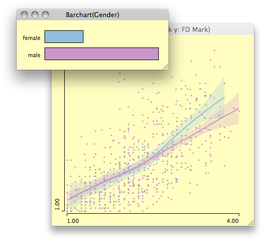
  • All smoothers can be plotted for subgroups, which have a color assigned, “smoother by colors“.
  • The color scheme has been refined once again, to make use of colors as efficiently as possible.
  • alpha-transparency is now consistent between scatterplots and parallel coordinate plots.
  • A new transformation: columnwise minimum and maximum.
  • Sorting of levels is now stable, i.e. levels which have the same value for an ordering criterion will keep their previous order.
  • The Reference Card speaks Windows now, i.e., Windows users no longer need to translate keyboard shortcuts from the Mac world.
Being able to use colors to estimate scatterplot smoothers for different subgroups is really handy – and actually “stolen” from early versions of DataDesk.
Principal curves are quite fun to play with, as there is no actual functional relationship needed, but the curve is generated such that the sum of the squared orthogonal distances to the curve is minimized. With no flexibility allowed this is obviously the PCA solution, with more and more flexibility the solution(s) get less obvious …
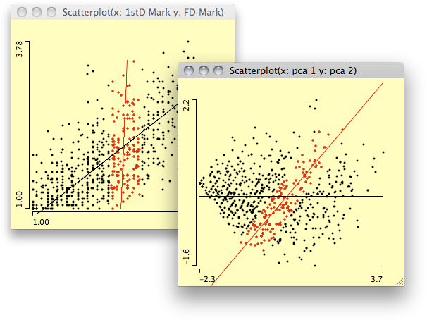
Above example shows the principal curve (actually the PCA-regression, left plot) and a linear least square fit on the first two principal components (right plot), which is actually the same line as in the left plot, only rotated to be a horizontal line. The highlighting in the left plot underlines, that principal curves are not following a functional relationship like y = f(x).
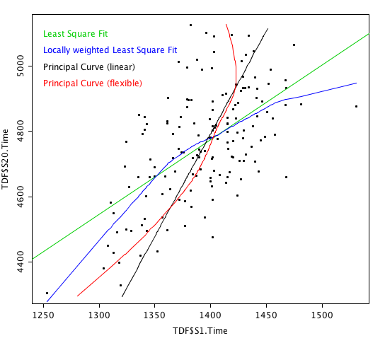
How different the various fits in a scatterplot can look like, can be seen here:
The plot shows the results of the 1st and the last time trial of the Tour de France in 2005. Depending on the type of rider we might expect the one or the other correlation between the two dimensions, and it is not too obvious, how the times should depend on each other.